OPTIMIZER GUIDE
StrategyQuant X
CONTENT
INTRODUCTION
Optimizer is the last ring of backtests that can be applied to the generated strategies to test their robustness and effectiveness. Its idea is to find the most optimal values for a strategy through series of backtests. This is achieved by the three types of optimization tests developed by StrategyQuant.
Optimizer has three main sections on its main screen:
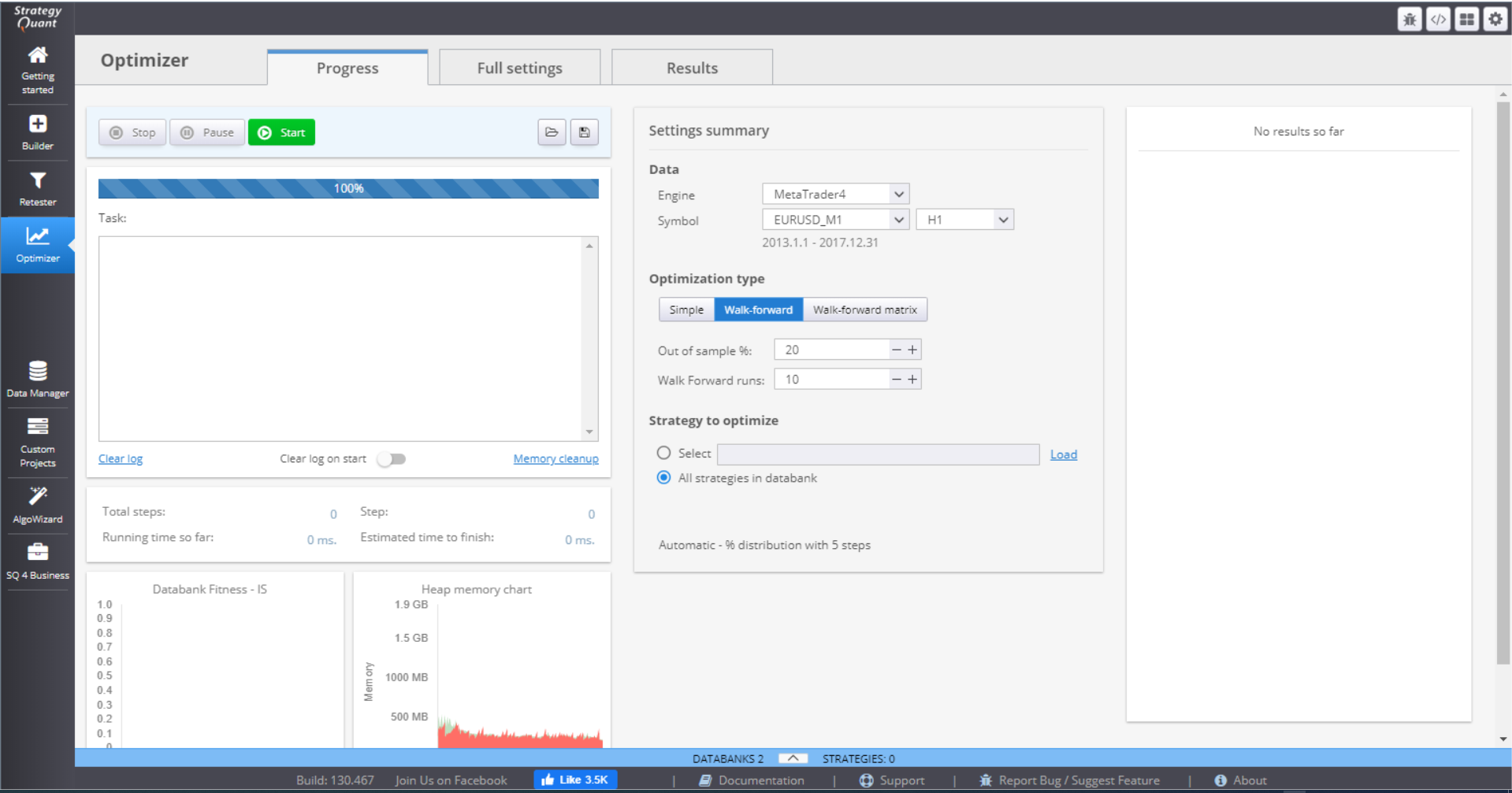
Progress (Engine) tab – this is where you can start or stop the task and follow its progress. You can monitor the statistics or quickly change a setting.
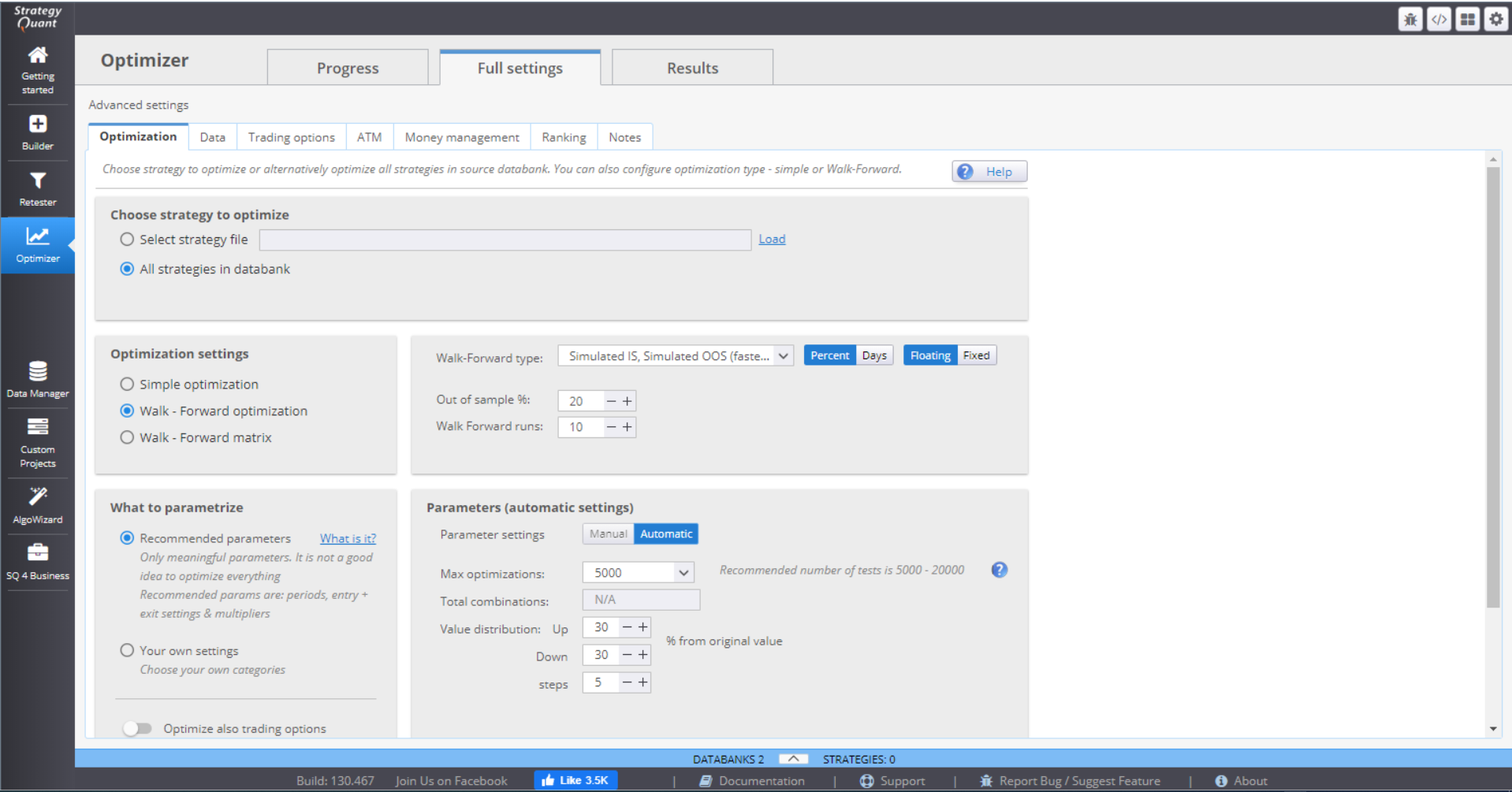
Full Settings tab – these are all the settings that can be configured for the optimization of your strategies.
Results tab – shows a variety of charts and tables of the strategies, their optimization results and statistics.

PROGRESS SECTION
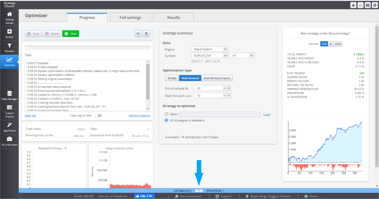
This section shows a summary of the settings applied to the current strategy optimization process and the overall progress, as well as a summary of the results. The first part of the screen contains a log where you can see which strategy is being optimized and what is its assessment according to the optimization criteria.
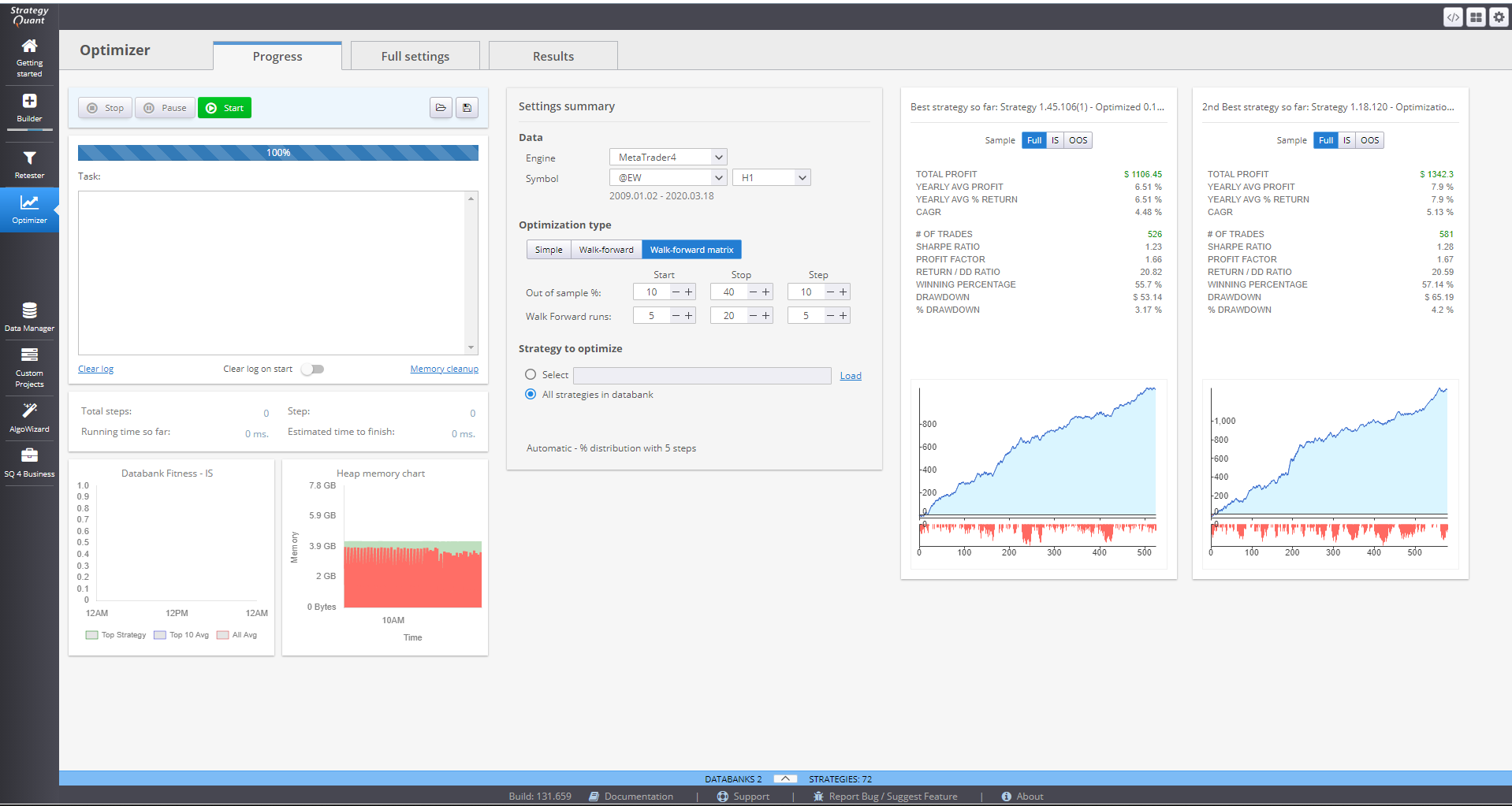
You can Stop, Pause and Start the optimization process using the buttons on the top of the section. You can Load settings, or Save your progress.
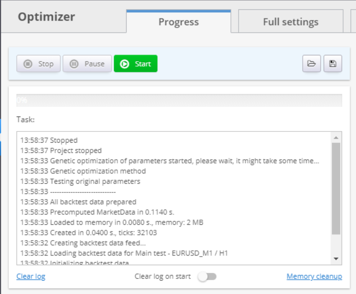
There is a summary of the optimized strategies that gives details about the total steps in the optimization plan, steps taken so far, running time since start and estimate of the remaining time.

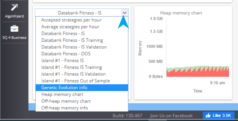
The charts on the bottom are configurable so you can choose what to see.
You can make some quick adjustments to the settings in the Settings Summary part. There is info about the Trading engine, the symbol data and the timeframe. You can quickly change the optimization type here.
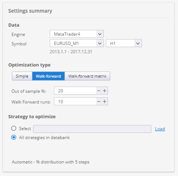
Strategy to optimize has two options. You can choose to optimize just one strategy by loading it into Optimizer, or you can process all strategies from the databank.
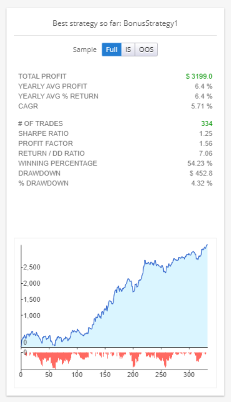
The third panel of the Progress menu is Results. You can see some statistics of a chosen strategy here. If you click on the panel, it’ll lead you to Results menu, where you can get full details of the strategy performance.
Databank can be accessed by clicking the arrow in the middle/bottom part of the Progress window. It stores the currently processed strategies.
You can perform multiple actions with the data. You can sort it using different parameter, save or load data.

If you double-click an item, its details are opened in the Results section.
FULL SETTINGS SECTION
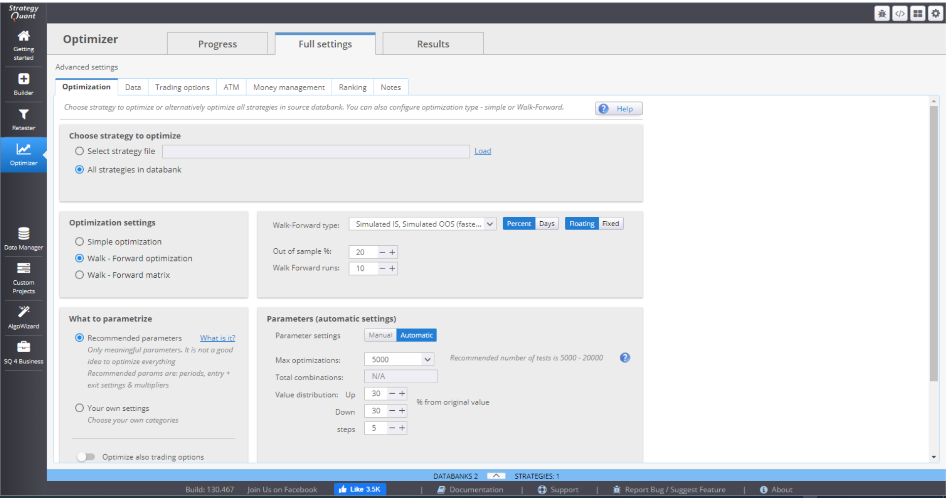
This is where you choose all components that would be included in the strategies optimization. You set their values, boundaries, conditions, restrictions.
OPTIMIZATION
This tab is the place to set the optimization parameters.

The first part is where you choose to optimize a selected strategy and load it, or optimize all strategies in the databank.

Optimization settings is where you choose the run process. You have three options.
› Simple optimization will test each parameter in a given range, to find the optimal performance of the strategy.

You can select to store all results in the databank or just the best candidates.
› The second option for optimizing the strategies is the Walk – Forward optimization. It divides the history data into pieces. Each piece has two segments – In sample (IS) and Out of sample (OOS). The first segment is where the actual optimization is done by testing each parameter in a given range, to find the optimal performance of the strategy.

Once optimized, the strategy is then tested on the OOS segment. This is history data unknown to the strategy and to Optimizer. It does not include the OOS period into the optimization process. This ensures an objective evaluation of the strategy performance.

Once the optimization of the first piece of history data is completed (IS + OOS parts), the algorithm takes the next step and performs the same tests on the next piece. To keep the optimization going further, it includes part of the IS segment and the whole OOS segment from the previous step to do the IS analysis of the current piece of history data.
› The last option is the Walk – Forward matrix. It takes the process one step further. It performs multiple Walk-Forward optimizations and tests different In Sample / Out of Sample configurations. By doing this it calibrates the effectiveness of the strategy in simulated real-trading environment. Because financial markets are a volatile, ever changing place, even the best strategy can lose its edge if it does not follow the dynamics of the market.


Regular optimization can be beneficial to a strategy, maintaining its robustness in the changing markets. The Walk-Forward Matrix answers the important question of how often re-optimization should be performed.
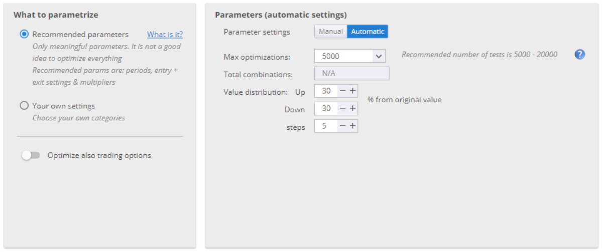
The next section of the menu is What to parametrize. It is where you configure the parameters that will be optimized. You can work with the recommended parameters, which are periods, entry and exit settings and multipliers.
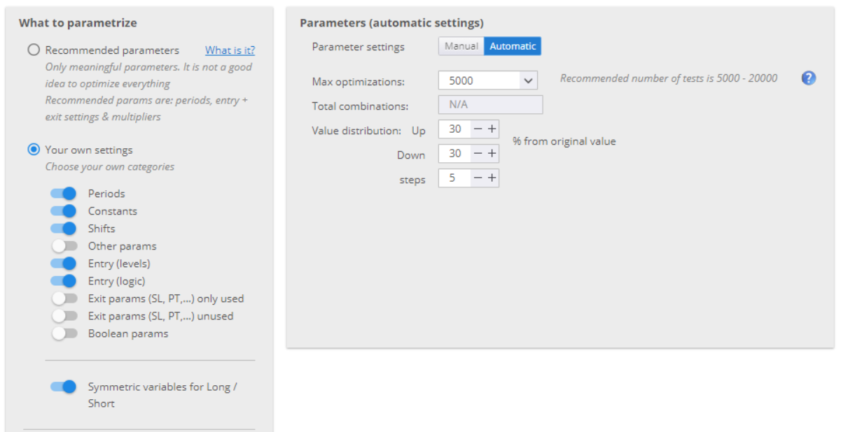
The other option is to choose your own categories for the parameters. If your turn on Symmetric variables for Long/Short the settings for long positions would automatically be mirrored for short positions.
You can optimize the trading options as well. These are the rules and ranges defined in Trading options menu.

DATA
This menu contains the settings for your backtests.
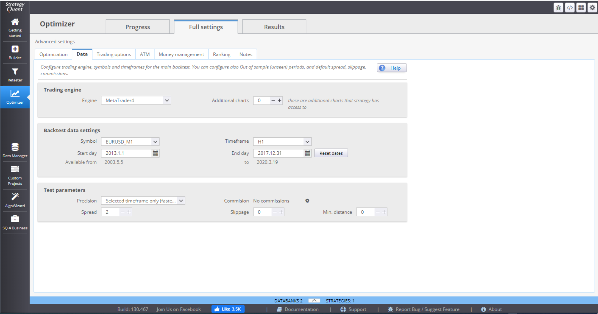
› In Trading engine, you can choose the trading platform that you want to work with and indicate how many additional charts you will use.

› Backtest data settings allow you to choose symbol, timeframe and time period for the backtests. There are separate settings for the main chart and for the sub charts.

› Test parameters - here you specify the precision of the data.

There are 4 options for setting the Precision:
› Selected timeframe only generates 4 ticks per bar – at Open, Close, High and Low for the period.
› 1 Minute data is more precise. It uses 1-minute data (if available) and generates 4 ticks per minute. This way it simulates price changes within the bar.
› Real tick – custom spread uses real tick data (if available) for the Bid price. It calculates the Ask price based on the spread that you specify.
› Real tick – real spread uses real tick data with real Bid and Ask prices. This is the slowest backtesting method of the four, so it should be used for final verification only.
You can choose to set the Commission rate.
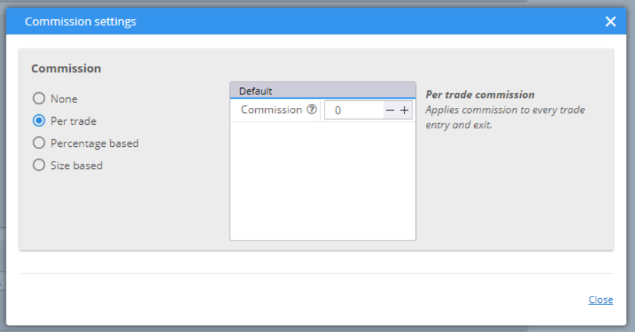
The Spread value would be used to calculate the Ask price if you choose Real tick – custom spread for precision method. Slippage adds a specified number of pips to the opening or closing price of your positions. Min.distance is set for your pending orders. Some brokers set limits on the distance from the current price when placing limit or stop orders.
TRADING OPTIONS
In Build and Trading options you can specify rules for the opening and closing of trades.
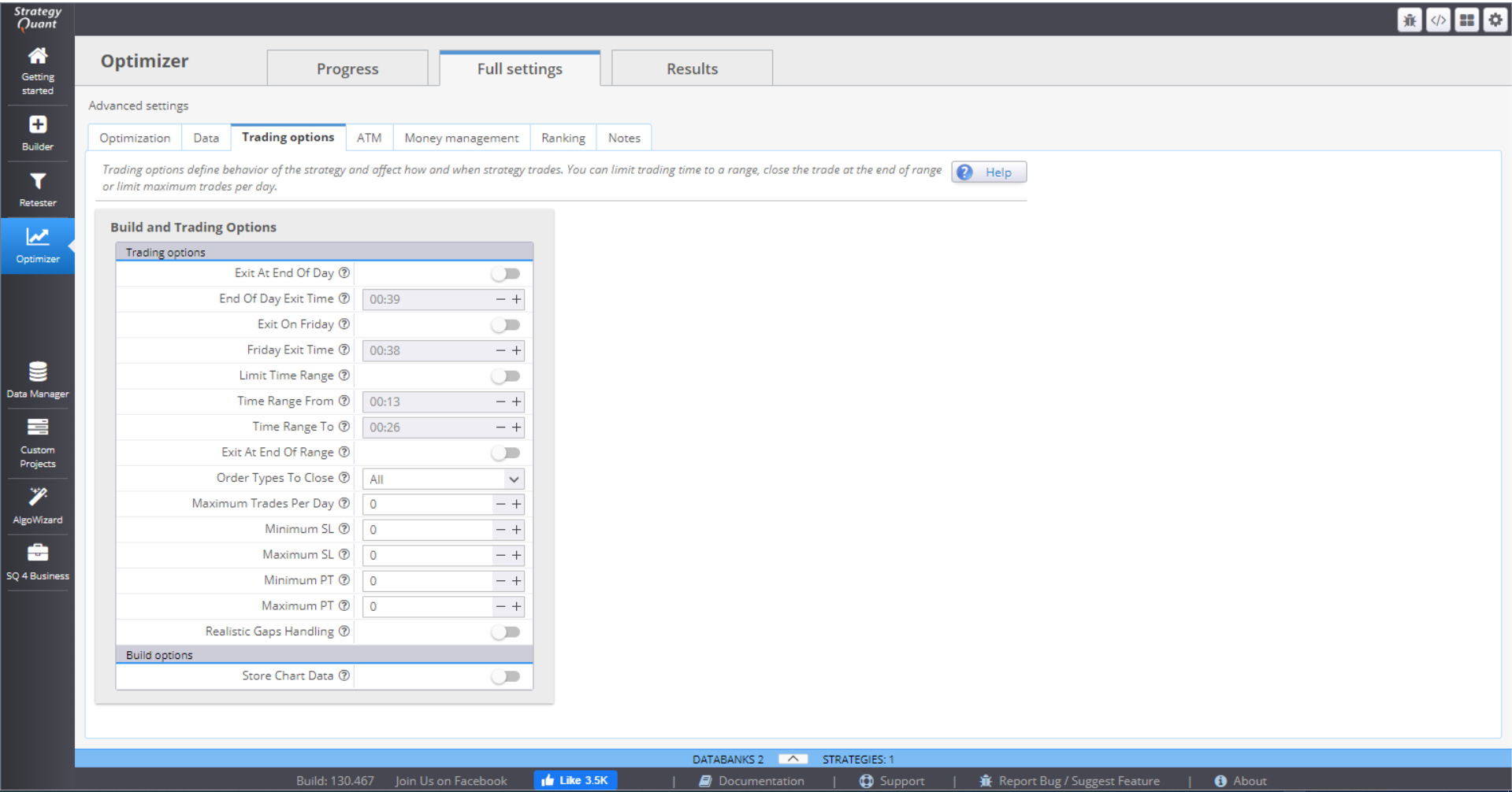
You can choose to exit all positions at the end of the day, or on Friday, and specify the exact time.
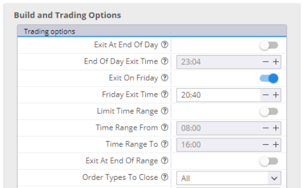
If you switch Limit Time Range on and fill in the range, the strategy will open trades in this time period only. You can choose to close the open positions at the End of the Range. You have the option to close all positions, live trades only or pending trades only. If you leave that inactive, the strategy will leave your positions open.
If you want to, you can limit the maximum number of trades per day.
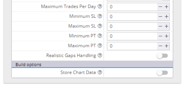
You can set minimum and maximum values for the Stop Loss and Take Profit orders. In this case, if the random generating process selects values beyond the range, they will be automatically cut to fit in. Zero in the value field means random value.
Realistic Gaps Handling is a way to handle gaps more realistically than the MetaTrader4 backtester. The latter would fill a pending order at its limit/stop price, which is not accurate. In real trading the order will fill at a price level after the gap.
If you choose to Store Chart Data, you will have complete chart data of your backtest, with all the indicators and all the trades on it.
ATM
The Advanced Trading Management allows you to configure multiple exits to your open positions. Using this option will disable all other exit options – Profit Target, Trailing Stop, etc. It will only use the Stop Loss settings and the ones configured here, in ATM.
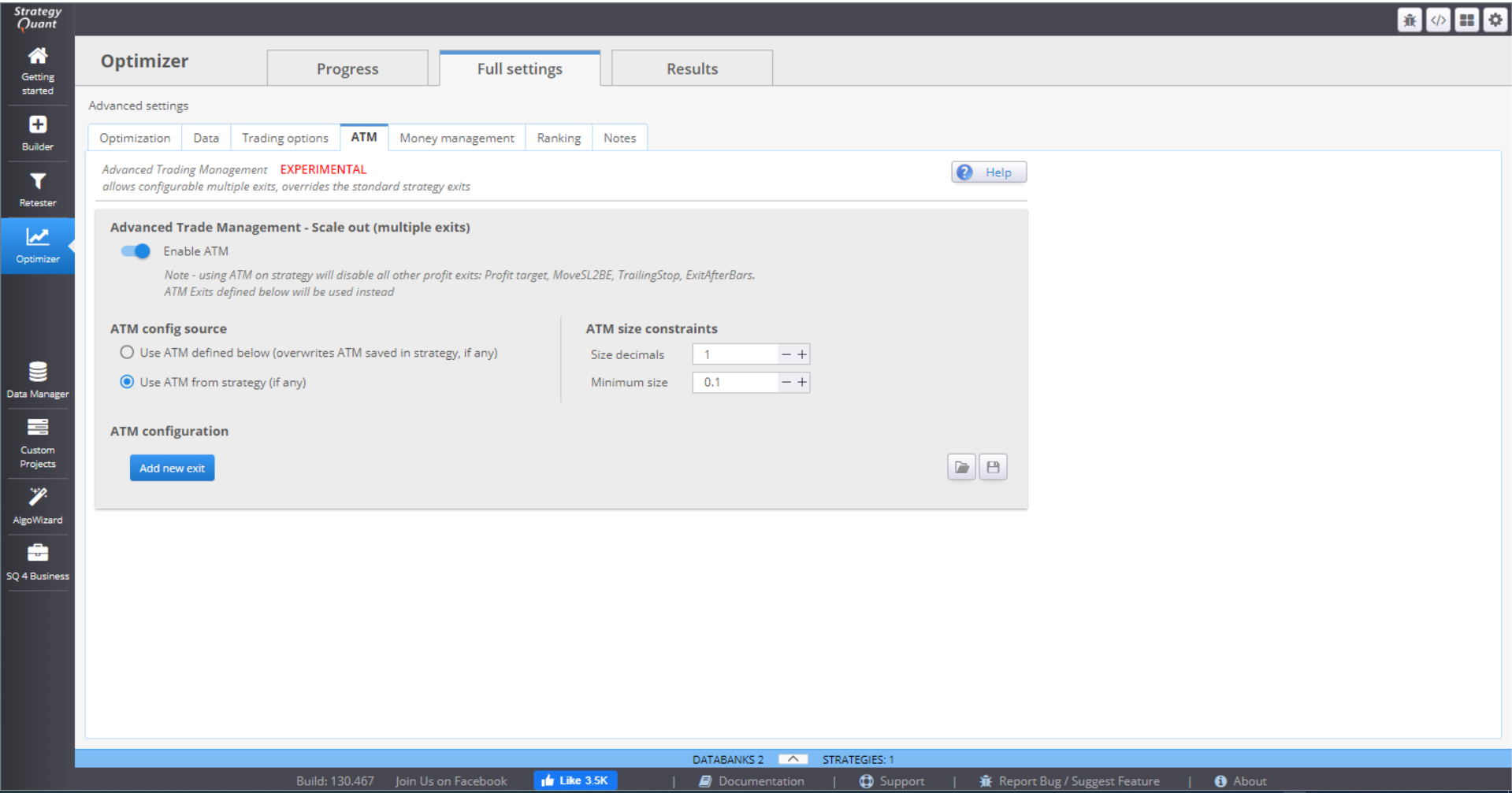
The idea is to close one part of the trade quickly after the profit is enough to cover the costs and the risk. The other part of the trade is left open to reach further profit target(s).
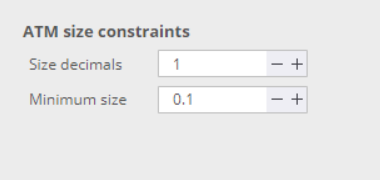
ATM size constrains gives some rules to ATM when computing the position parts. Size decimals gives instructions how to round the parts size. Minimum size is the smallest acceptable size of one part.
Then you need to configure the rules by clicking the Add new exit button.
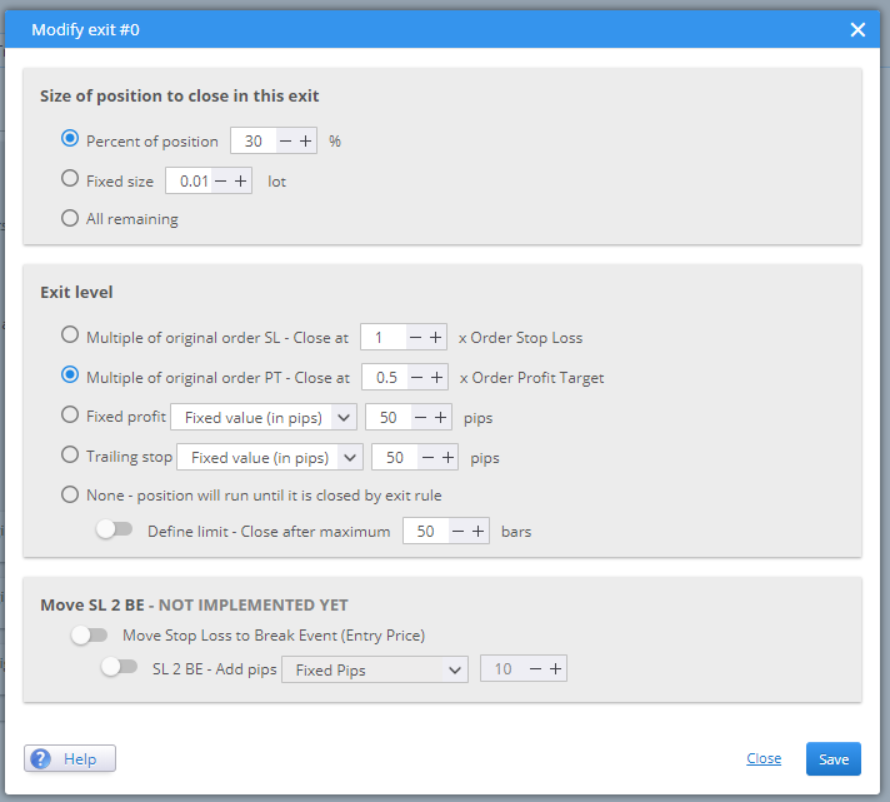
Size of position to close in this exit gives you three options. Choose whether you want to compute the parts using a percentage or a fixed size. All remaining is suitable for setting rules for the last part of the position.
Exit level is where you define when you want this part of the position to be closed. You can set it to be dependent on the SL or TP. Or choose it to be a fixed value. The last option is to close the part after a given number of bars.
When you configure the rules, they are saved and applied to your strategy.

MONEY MANAGEMENT
In this menu you configure the initial capital and the position sizing method.
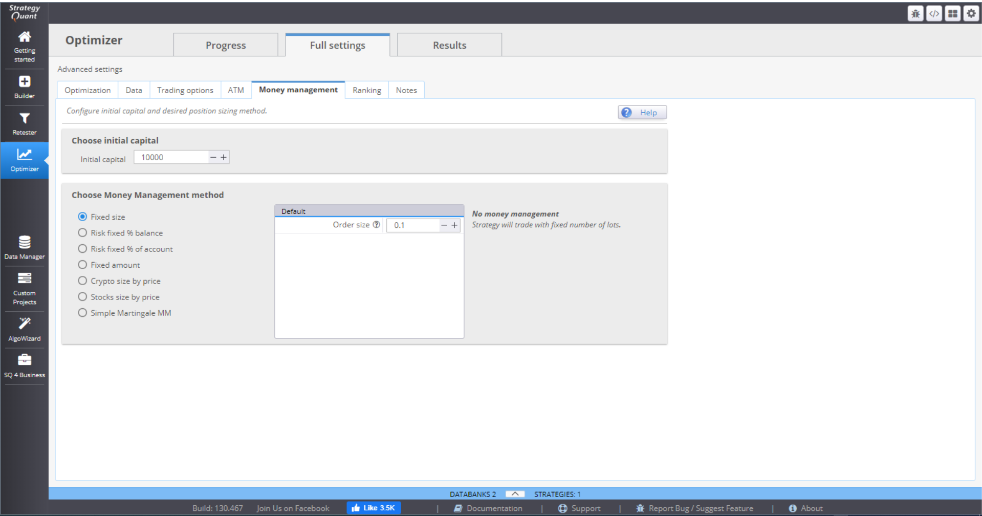
There are 7 MM methods to choose from:
⇒ Fixed size – the positions are opened using a fixed number of lots. This simple method is good when generating new strategies, as it gives you a clear overview of its real performance.
⇒ Fixed % of balance – this method will risk a certain percentage of your balance, meaning the money that you have in your account without including the profit/loss from open positions.
⇒ Fixed % of account – this will risk a certain percentage of your equity. The difference with the previous method is that the position size is calculated on balance, including profit/loss from open positions. This makes the method extremely sensitive to account changes, which is very effective money management.
⇒ Fixed amount – this method risks a fixed amount every time. It is a good way to test a strategy with Stop Loss, based on volatility (ATR), or when you want to compare strategies with different SLs.
⇒ Crypto size by price – this method is designed for crypto trading. You need to specify the exact number of characters after the decimal point that will be used. The initial capital is used by default, but you can set the method to use the account balance.
⇒ Stock size by price – the method is designed for trading stocks. Like the crypto method, the initial capital is used by default, but you can choose to use the account balance.
⇒ Simple Martingale MM – this method starts from a fixed size (in lots) and increases the position size by a set multiplier after each loss. The size is reset to starting point when the trade is closed for profit, or when the size exceeds a defined maximum size (in lots). There is an option to use separate logic for buy and sell orders.
RANKING
After the strategies are optimized they are given a rank, depending on their results. This rank is a number between 0 and 1, and is a representation of the strategy’s fitness (quality), or how well it performed, according to predefined criteria.
This section is where you define how the strategies are rated. You can also configure filters to further evaluate the strategies before they are saved in the databank.
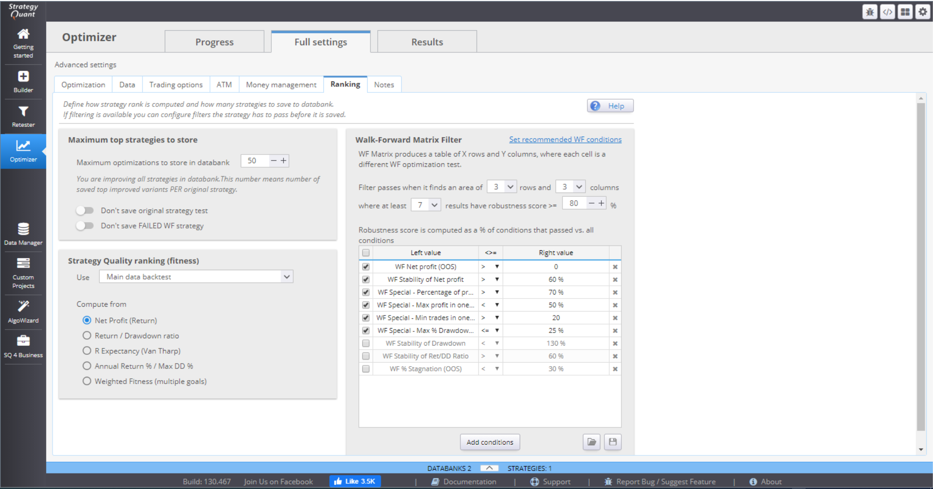
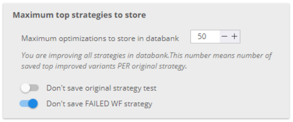
You can set the maximum number of strategies that will be stored in a databank. If you are improving all existing strategies from the original databank, the number means how many top optimized candidates per original strategy will be stored into the new databank.
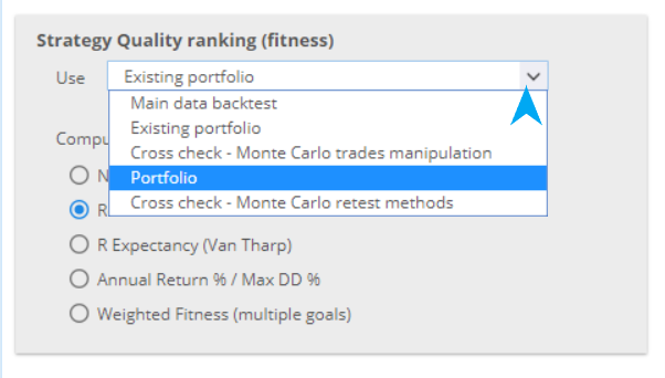
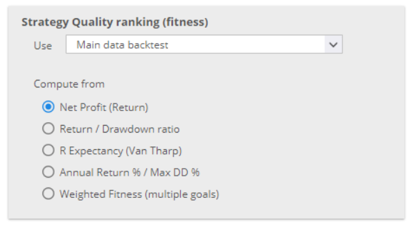
You can choose the data that will be used to compute the fitness.
Then you can select the criteria to use for the ranking. You may choose one of the default computations.
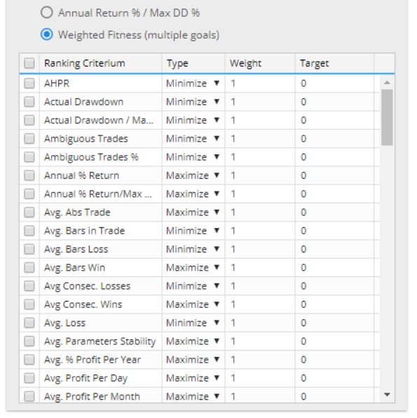
Or, you can configure custom rules. The options here are flexible and you can set the rules in a variety of ways.
The filtering criteria can be set by default or you can customize the values. The Walk-Forward matrix produces results that are plotted on 3-D diagrams in Results, where each cell, formed by the measuring units of the X and Y axis, represents one test.
For the purposes of this analyses, a robustness score is computed. The conditions that need to be passed are manageable. The rate of the robustness score is measured by the part of them being successful.
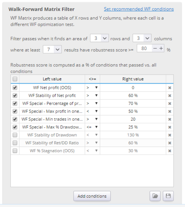
A Walk-Forward matrix optimization is considered successful when a defined number of individual tests (in a range, sized by you) obtain a better robustness score than the minimum percentage that you have selected.
NOTES
You can write down your notes here. They will be saved together with all configuration settings of your project.
RESULTS
Results provide a wide variety of statistics in different forms – charts, diagrams, tables.
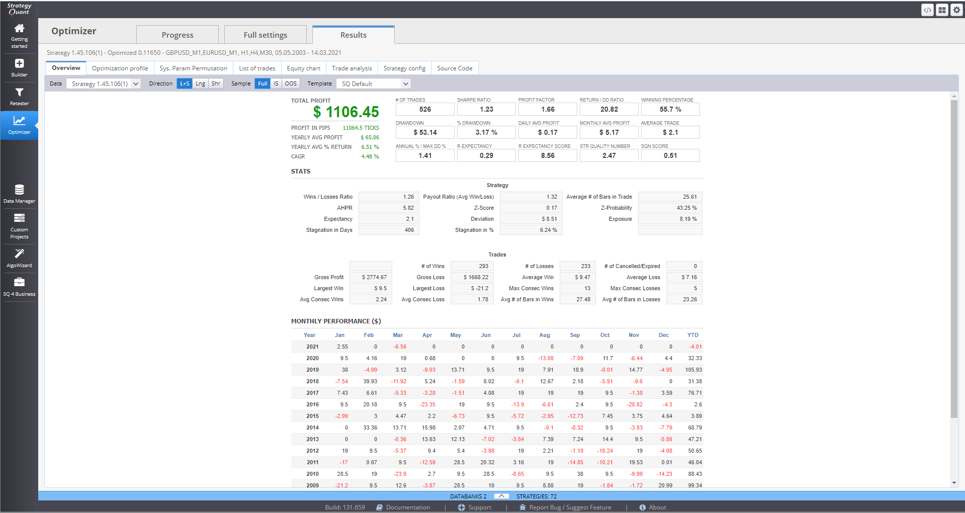
Overview tab shows detailed statistics and the monthly performance of a strategy.
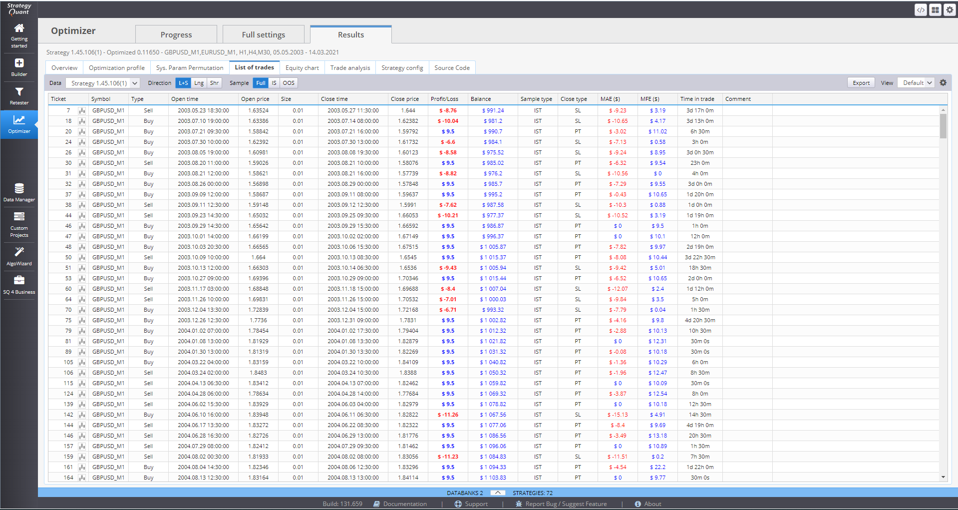
List of trades holds information of every strategy, recorded in the databank.
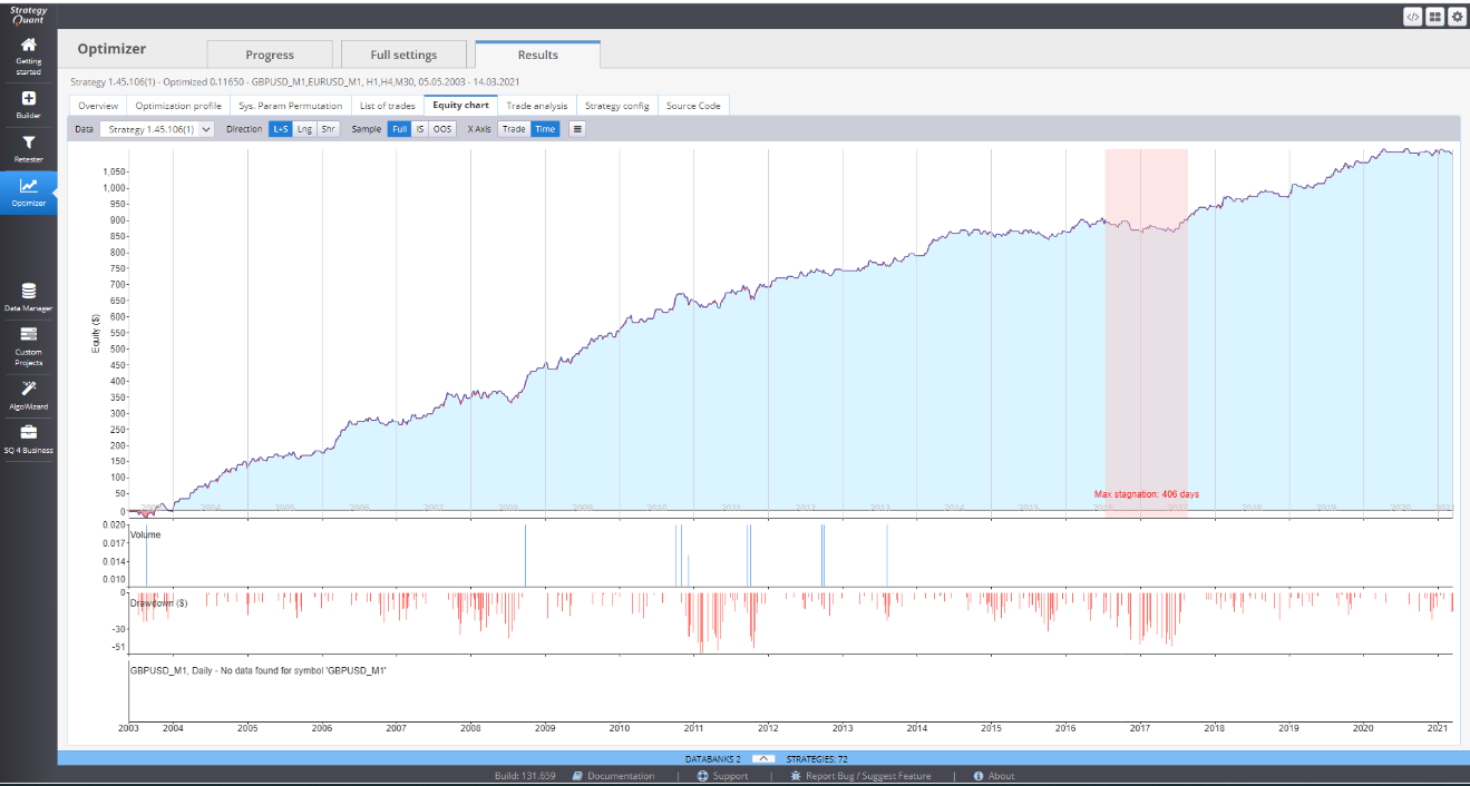
Equity chart can visualize the equity curve of a strategy.
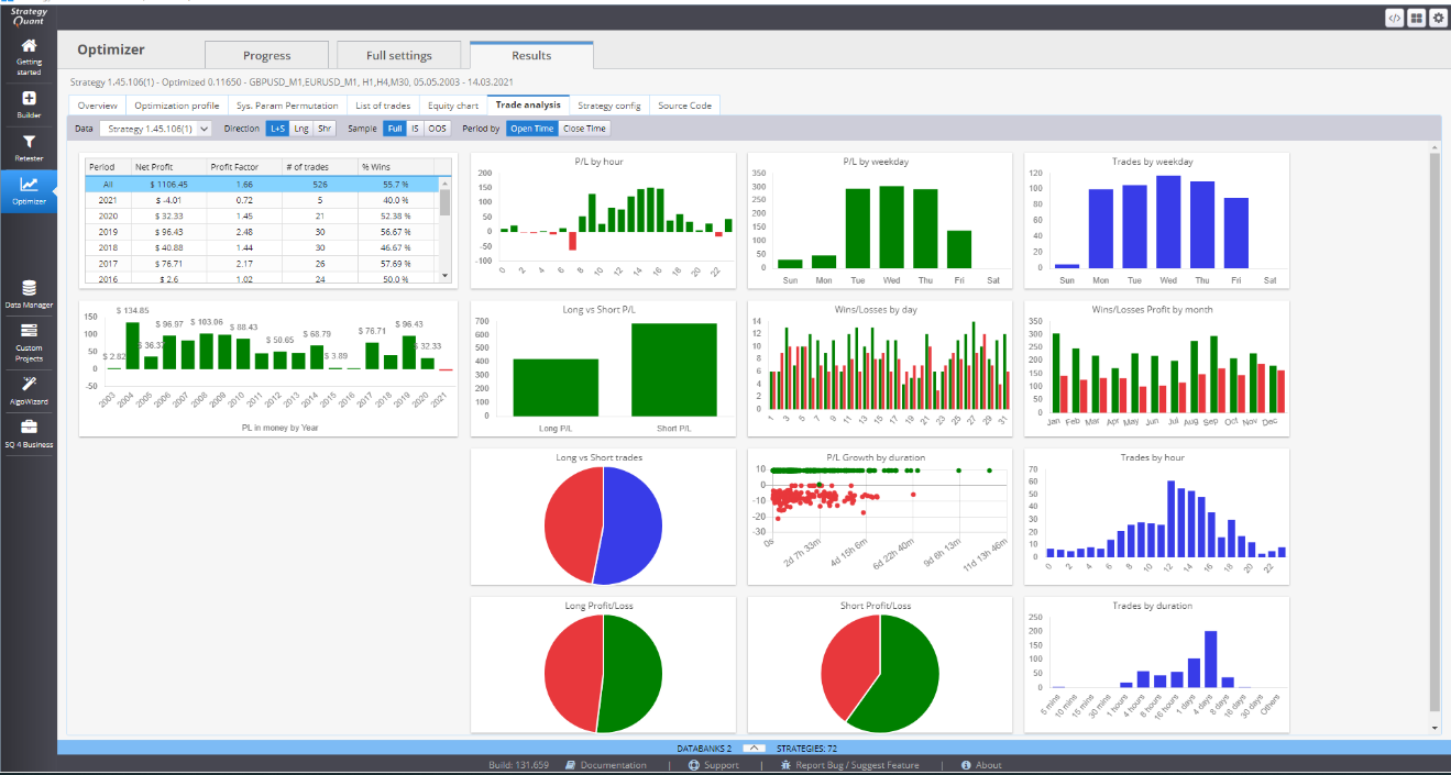
Trade analysis contains multiple charts for the performance of one strategy.
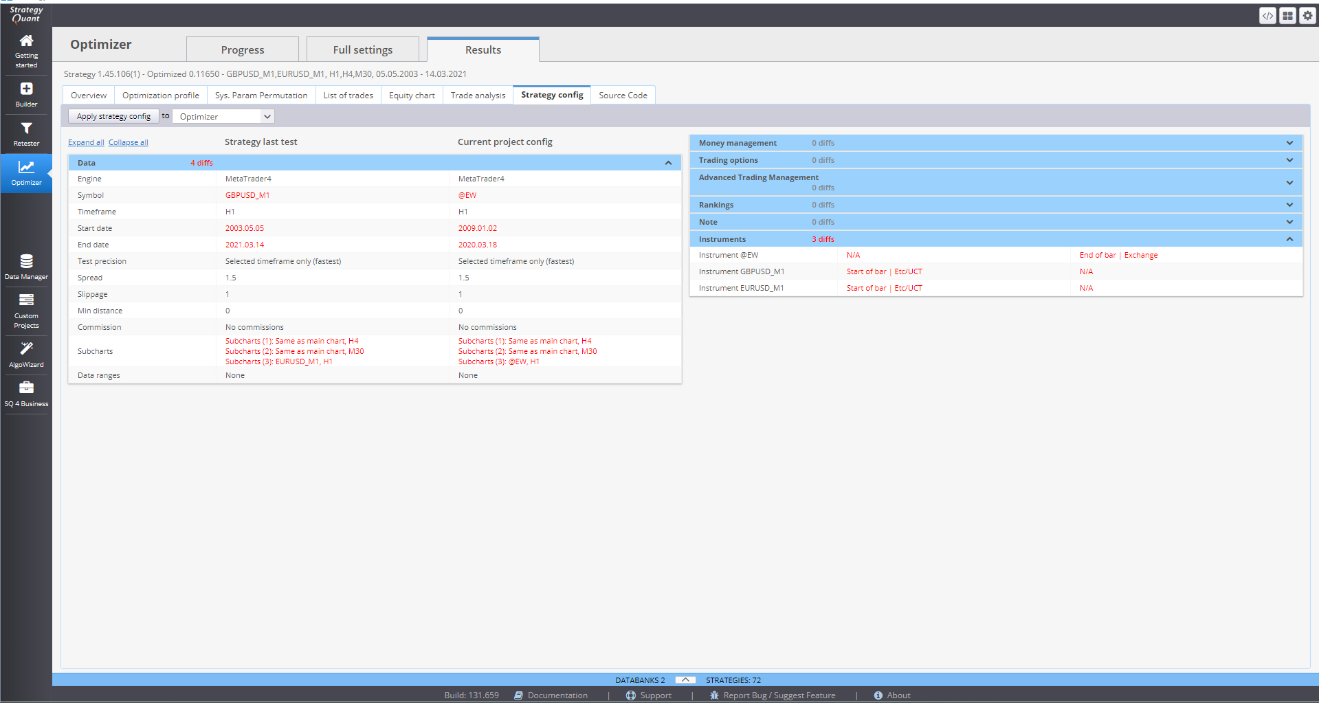
Strategy config is an overview of the current settings.
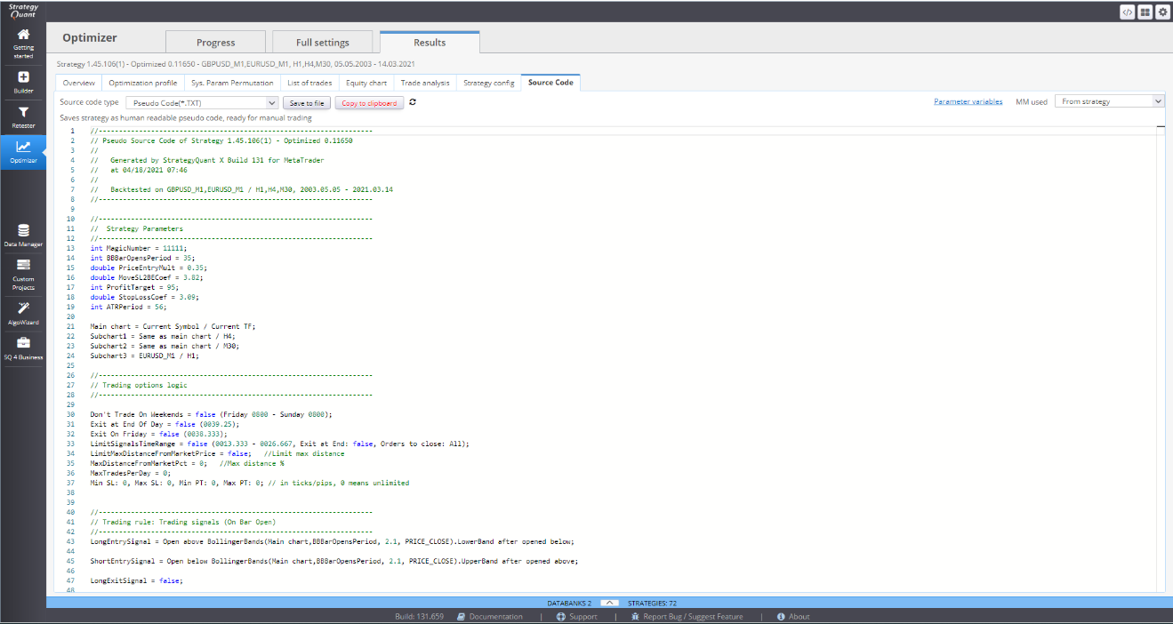
Source code is where you can get the complete code for your strategy. There are several options for how to view it. You need to select the right trading platform, so that StrategyQuant generates the proper code. You can then copy it, or save it to a file and upload it to your trading platform.
